Breast cancer cell statistics · Amirassyl Sagyndyk

The dataset has 569 biopsies, each described by measurements of the cell nuclei and labelled malignant (212) or benign (357).

Do malignant tumors differ in cell symmetry?

I compared mean cell symmetry between the two groups with a two-sample t-test, a 95% confidence interval, and Cohen’s d. The descriptive statistics (mean, median, mode, standard deviation, range) are written from scratch instead of taken from a library.

Result	Value
Mean symmetry, malignant vs benign	0.1929 vs 0.1742
t statistic	8.34 (p = 5.7 × 10⁻¹⁶)
95% confidence interval for the difference	[0.0142, 0.0233]
Cohen’s d	0.72 (medium)

Malignant tumors have a higher mean symmetry value. The difference is statistically significant with a medium effect size.

How well does tumor radius predict concavity?

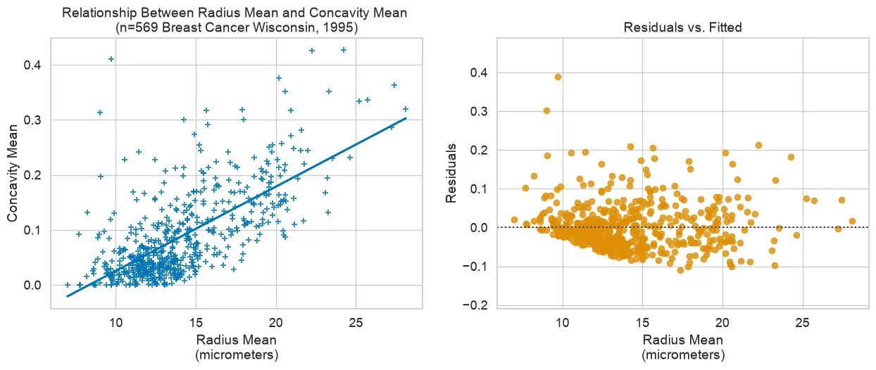
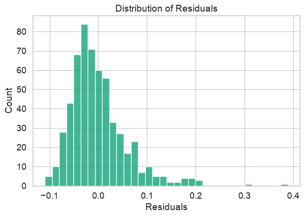
I fitted a simple linear regression of mean concavity on mean radius, then checked the model’s assumptions with a residuals-vs-fitted plot, a residual histogram, and a normal Q–Q plot.

Result	Value
Pearson’s r	0.677
R²	0.458
Regression line	concavity = 0.0153 × radius − 0.1275
Slope, 95% confidence interval	[0.014, 0.017] (p = 1.9 × 10⁻⁷⁷)

Radius explains about 46% of the variation in concavity. The slope is clearly non-zero, but the residuals are right-skewed: concavity cannot go below zero, which puts a hard lower edge on the residuals while a few tumors sit far above the line. The normality assumption does not fully hold, and I say so in the write-up.

Two panels. Left: scatter plot of mean concavity against mean radius in micrometers for the 569 tumors, with an upward-sloping fitted regression line. Right: the residuals plotted against mean radius, with most points in a dense band just below zero and a scattering of points far above it.

Histogram of the regression residuals. Most fall between −0.1 and 0.1 with the tallest bars just below zero, and a thin tail extends to the right as far as about 0.4.

Background

The notebooks started from a course template, and the regression plotting helper follows the template’s structure. The analysis, statistics functions, and interpretation are my own.